Getting Starting with Excel Formatting

When it come to Excel formatting, there are so many options and tools that it can be a little overwhelming trying to determine what to use and how to use it. Luckily, there are some beginning steps that can help you focus on where to begin.
Special Paste
In the following article, we will start with some of the more basic tools and features you can use and then get into an Excel formatting macro as a suggestion on something you can do once you’re comfortable with the basic stuff.
Freezing Column Headings
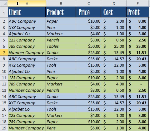
When you’re working with a long excel spreadsheet, you might want to see what your column headings are so that you don’t have to keep scrolling up or make a mistake.
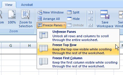
To make this easy, freeze the column headings. This will always keep your first row with the headings at the top of the columns regardless of how far down you scroll.
To set this, click on “View” on the tool bar, and then select “Freeze Panes.” Click on the “Freeze Top Row” option.
Quick Tips For Adjusting Columns and Rows: Your Handy Excel Formatting Cheat Sheet
- To quickly insert a column or row, select the row or column by clicking on a corresponding cell, then click “Ctrl” and “+”
- To quickly delete a column or row, select the row or column by clicking on a corresponding cell, then click “Ctrl” and “-”
- Autofit makes the columns big enough to fit their contents. To do this, select the column(s) that you want to change, then click on the “Format” icon on the tool bar and select “AutoFit Column Width.”
- Another way to adjust the column size is to fit it to the text you enter. To do this, first enter your text, then double click the separating line between that column and the column to the right of it. The column will enlarge to fit the text.
Key Board Shortcuts to Help you Save Time in Excel Formatting
- “Ctrl” + “b” à Bold
- “Ctrl” + “i” à Italic
- “Ctrl” +” u” à Underline
- “Alt” + “=” à Auto Sum
Formula Tricks for Quick Excel Formatting
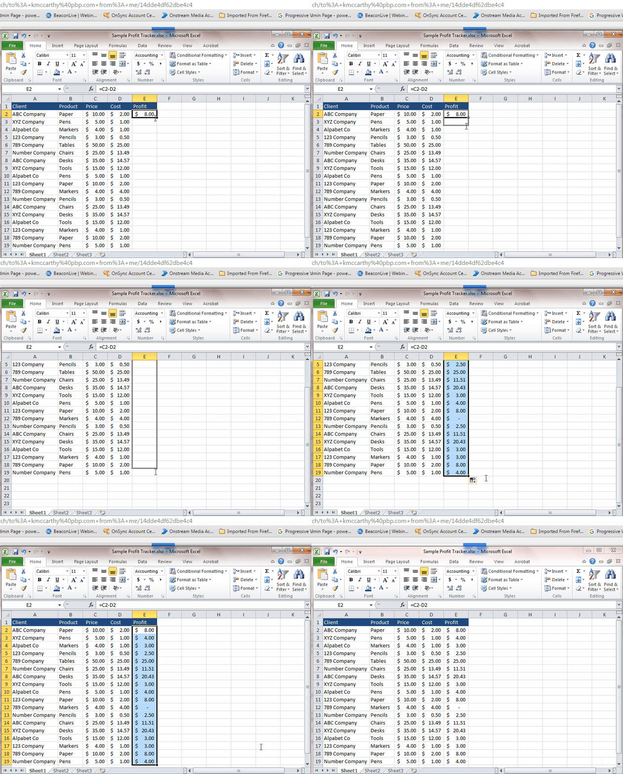
To copy a formula down the length of a column, click on the cell with the formula. Then, put your cursor in the bottom right corner of the cell until you get the thick, black plus sign, you can either drag the formula down or double click and the formula will be copied down the length of the column.
However, keep in mind that this will adjust the formula in each row to correspond to the data, in the same row as the formula. So, if you have a value that will stay the same in each formula you must add “$” before the letter and in between the letter and the number of the cell you want to keep the same (for example, $A$1)
Excel Formatting Macros
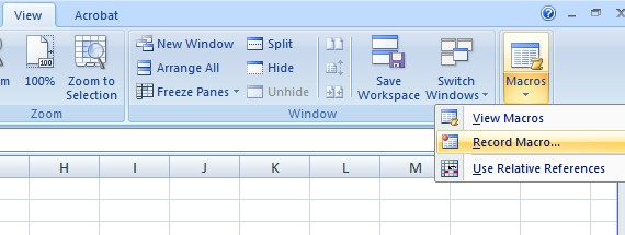
Sometimes, using a Macro can help you save time in Excel formatting. To create formatting macros, first select the cells that you want to format. Then go to the “View” tab on the tool bar. Click on “Macros,” then select “Record Macros.” You will be prompted to name and provide a description of the macro.This could be useful in a spreadsheet where you are using multiple macros. Record the keystrokes to format the cells that you have selected. When you’re finished go back to “Macros” and select “Stop Recording.”
To use the macros you recorded, go to “Macros” and select “View Macros.” You will get a list of all the macros you recorded. Select the one you want to run and then click “Run.”
We here at Learn Excel Now hope you feel more comfortable using formatting.
Getting social with Excel: please feel free to share this article with anyone you think would benefit from it.
Kevin – Learn Excel Now


