Excel Time-Saving Formulas: Quick & Easy Tricks to Work More Efficiently

As any user knows, Excel offers a huge variety of formulas and functions for processing calculations. However, searching and finding each one can be time-consuming. The following Excel time-saving formulas will help you quickly process the information you need so you can focus on your work.

AutoSum

The autosum feature is a great shortcut for quickly adding up columns and rows of numbers in Excel. To use it, click on the last cell in the row or column that you want to find the sum of and click on the autosum (sigma) button. A blue dashed-line box will outline the data that Excel thinks you want to include. If you need to make adjustments, simply drag the blue dash-lined box to hold the data that you want. When you have verified that this is the correct data, push enter.  The sum of your column of your row or column will appear in that cell.

Goal Seek

Goal Seek is great for finding an input, by working backwards and defining an output in order to figure out what input you would need to enter. It saves you time from having to use a trial and error method. To use this feature, first enter your data in a spreadsheet. Next, you will need to click on the cell that you want to change. Go to the “Data” tab and click on the “What-If Analysis” and select “Goal Seek” from the drop-down menu. The goal seek dialog box will pop up and you can enter your values. The “Set cell” box will contain the cell that you clicked on originally (where the answer will go). In the “To value” box, enter the result that you want the data to align with. In the “By changing cell,” highlight the cells that you want to change in order to produce the result that you want. Click “Ok” and the goal seek status dialog box will appear. It will give you the solution that it found, but listing your “target value” and current value that it calculated. If you are satisfied with the result and want it to replace the original data, click “Ok.”

Concatenate

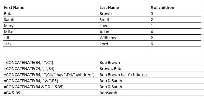
The concatenate feature allows you to join together two or more cells into one. For instance if you have data where one column has first names and another column has last names, you can use this feature to join them together in one column. Click on the cell that you want to enter the new value in and then enter your formula =CONCATENATE( ). Between the parentheses, you need to enter the cells that you want to join together.

Examples of formulas:

We here at Learn Excel Now hope you now feel confident in your ability to use Excel time-saving formulas. It is our desire to bring you the best advice possible to effectively and efficiently use your desktop features so you can focus on your work. Subscribe to our blog to receive weekly Excel tips. If you’re looking for more in-depth training check out our upcoming instructor-led, live online trainings.

Liked these Excel formula tips? Have questions? Leave your comments below; we’d love to hear from you.

Getting Social with Excel: Spread the word and share the knowledge!

Kevin – Learn Excel Now