One of Excel’s advanced functions is the RANK function. This formula is used to rank numbers in a dataset by either ascending or descending order.

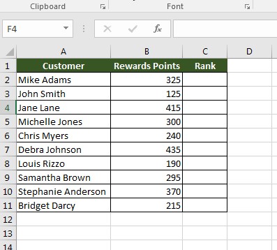
Let’s say you were running a customer loyalty program based on earning points. You need to rank customers’ point totals to determine what rewards they receive. You could do a simple sort, but your boss wants the customer names to stay in the same order.

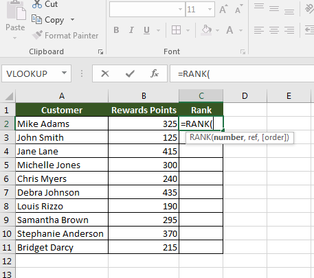
This is the example we will use:

You will use the RANK function for this challenge, but let’s first explore how the function works.

Syntax of the Rank Function

=RANK(Number, Ref,[Order])

When you use the rank function, your first argument is the number. This is where you specify the cell containing the number you want to be ranked. Next, you identify the range of numbers to be used as the reference (Ref). Finally, you select the order, which is ascending or descending.

Solving the Challenge

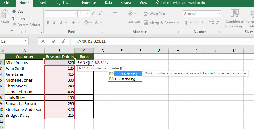
So, we will identify B2 as the cell to be used. Then, identify the range as B2 through B11:

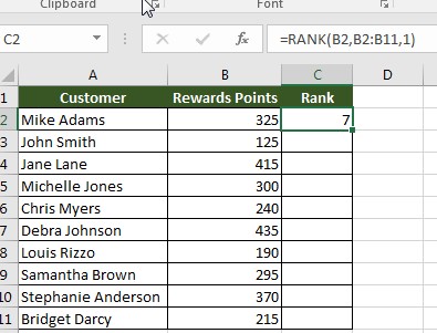
Then, select Ascending order and we get our first result:

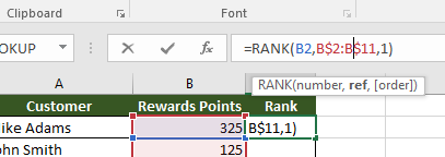
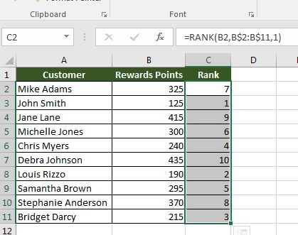
Before moving onto the remaining lines in the table, we need to add absolute referencing to the range so that it stays consistent while the number being compared changes for each line. A reminder to use the $ between the letter and number of the cell for absolute referencing:

Once you’ve added the absolute reference, you can now copy and paste the formula all the way down to reveal the rank for all lines:

We at Learn Excel Now hope you feel comfortable using the RANK function after this article.

Like Learn Excel Now? Follow us on social media and share our content with your networks! And don’t forget to sign up for the Newsletter

Kevin – Learn Excel Now